A team hands you a training job and a model server. The training job wants eight GPUs on one node, all at once, or it wants nothing. The model server pulls a 14 GB container image, then downloads 140 GB of weights before it answers its first request. Your Horizontal Pod Autoscaler, tuned over three years to add replicas when p95 latency drifts, adds a pod that takes four minutes to become useful by which time the traffic spike is over.
This is the point where most platform teams discover that AI infrastructure is not web infrastructure with bigger instances. The primitives look familiar (containers, schedulers, object storage, service meshes) and the failure modes are not. This guide walks the layers that differ, says what breaks, and gives you the decision rules worth having before the first GPU node joins your cluster.
The layers that make up AI infrastructure
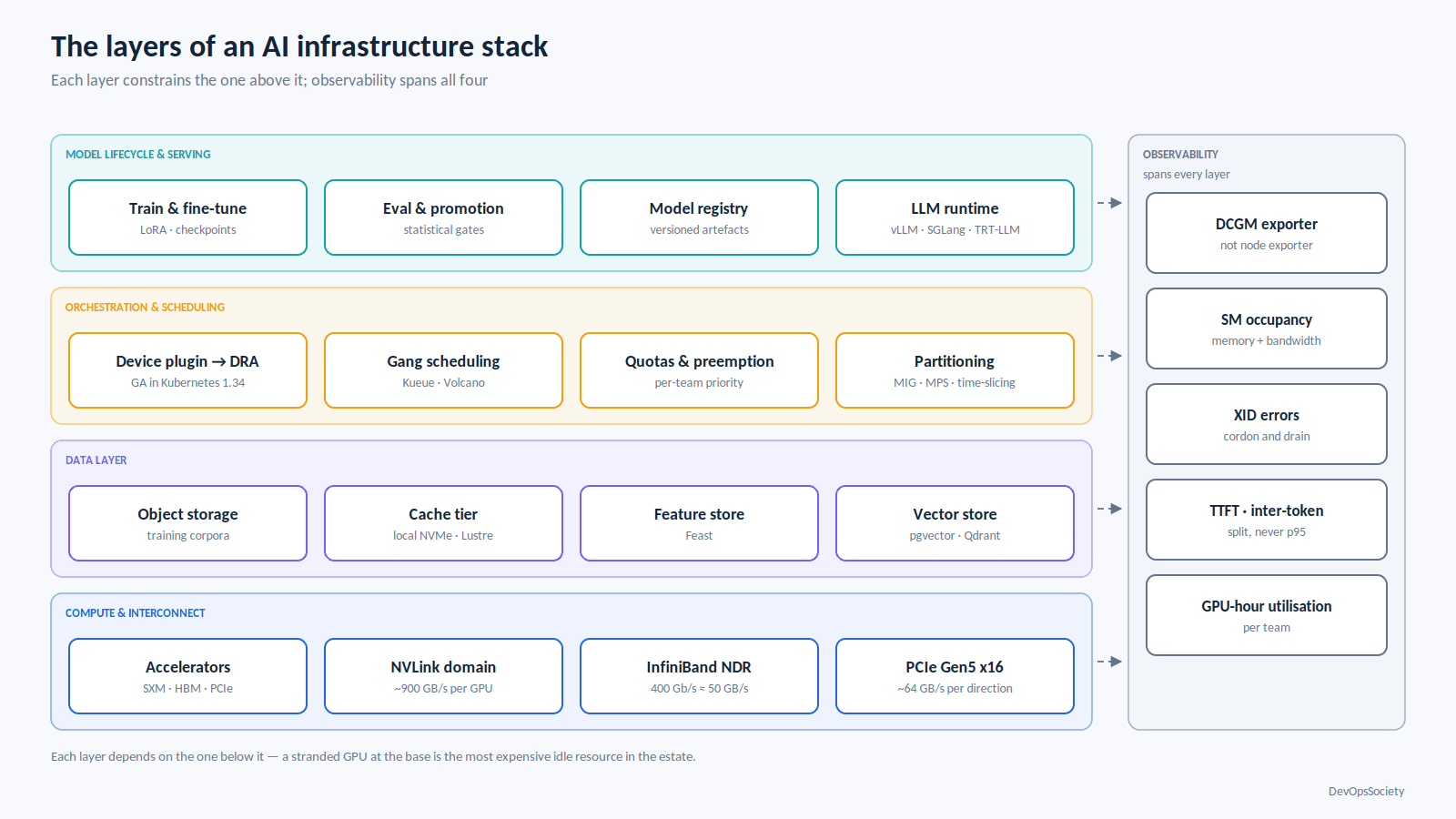
Strip away the vendor taxonomies and an AI infrastructure stack has five parts: accelerated compute and the network between accelerators; a data layer that has to serve both bulk sequential reads and single-digit-millisecond lookups; orchestration and scheduling that can place indivisible, expensive, topology-sensitive resources; a model lifecycle that spans training, fine-tuning, evaluation and promotion; and serving plus observability for workloads whose health signals are nothing like an HTTP error rate.
Everything else experiment trackers, model registries, prompt management, guardrail proxies sits on top of those five and is comparatively easy to swap. The five below are the ones that constrain your architecture. More on how they fit together across the rest of the AI infrastructure coverage on this site.
Compute: memory bandwidth is the constraint, not FLOPS
Spec sheets sell FLOPS. Your bottleneck is almost always memory bandwidth.
Transformer inference at batch size one is memory-bound: every generated token requires reading the entire set of model weights out of high-bandwidth memory. A 70-billion-parameter model in 16-bit precision is about 140 GB of weights. At 3.35 TB/s roughly what an H100 SXM delivers from its 80 GB of HBM3 the theoretical ceiling is around 24 weight-passes per second per GPU before you have done any arithmetic at all. That number, not tensor-core throughput, sets your tokens-per-second floor. It is also why the generational jumps matter in the way they do: the H200 moves to 141 GB of HBM3e at 4.8 TB/s, and B200 to 180 GB at up to 8 TB/s. Capacity decides what fits; bandwidth decides how fast it runs.
Two consequences follow immediately.
GPU memory is a hard wall, not soft pressure. When a pod exceeds its CPU request, the kernel throttles it. When a process exceeds GPU memory, CUDA raises an out-of-memory error and the process dies. There is no swap, no page cache, no graceful degradation. A model that needs 82 GB on an 80 GB card does not run slowly; it does not run. This single fact reshapes capacity planning: you size for peak resident memory (weights, activations, KV cache, fragmentation headroom), not for average.
Quantisation is a capacity decision, not just a performance one. Dropping from 16-bit to 8-bit halves the weight footprint and roughly halves the bandwidth needed per token. Whether the accuracy cost is acceptable is the ML team's call, but the infrastructure consequence is yours to model, because it changes how many GPUs a deployment needs.
Choosing a GPU class
For training and large-model inference you want SXM-form-factor datacentre parts with HBM and NVLink. For smaller models, embedding generation, batch scoring and most computer-vision inference, a PCIe card with GDDR memory (an L40S or L4 class part) is dramatically cheaper per unit of useful work, and the lack of high-speed interconnect does not matter because nothing is being sharded across devices.
The rule worth internalising: if the model fits comfortably on one GPU, buy the cheapest GPU it fits on. Multi-GPU sharding is a last resort, not a default, because it introduces a synchronisation cost on every forward pass.
Interconnect decides your topology
When a model does not fit on one device, the GPUs must exchange activations or gradients constantly. Inside a node, NVLink gives Hopper-class GPUs around 900 GB/s of aggregate bandwidth per GPU, and Blackwell roughly doubles that. PCIe Gen5 x16 gives you about 64 GB/s per direction. Between nodes, InfiniBand NDR runs 400 Gb/s per port, which is 50 GB/s an order of magnitude below intra-node NVLink.
That gap is why the eight-GPU node is the standard unit of AI infrastructure. Tensor parallelism, which shards individual layers, is viable inside a node and painful across nodes. Pipeline and data parallelism tolerate the network better. If you are designing a cluster, the practical question is not "how many GPUs" but "how many contiguous NVLink domains", and whether your cloud provider's placement groups can actually guarantee them. The same locality thinking that shapes good production design on AWS applies here with the stakes multiplied, because a badly placed training job wastes hardware at a rate ordinary compute never approaches.
The data layer: three access patterns, not one
Web infrastructure mostly needs one storage profile: low-latency reads of small records. AI infrastructure needs three, and they conflict.
Training data is read sequentially, repeatedly, at high throughput. A training job streaming from object storage across many epochs will saturate a network link long before it saturates the GPUs, and an idle GPU during data loading is the most expensive idle resource in your estate. This is why serious training setups use a caching tier local NVMe on the GPU nodes, or a parallel filesystem like Lustre or a managed equivalent between object storage and the trainer. Getting this wrong shows up as GPU utilisation sitting at 40% with no obvious culprit.
Feature stores solve a narrower problem: making sure the feature values used at training time match the ones computed at serving time. Feast is the common open-source choice, with commercial options above it. If your ML workloads are predominantly LLM-based rather than classical tabular models, you may not need one at all this layer earns its keep for recommendation and fraud-style systems, not for retrieval-augmented generation.
Vector stores are the newer addition and the one most likely to land on your desk unannounced. They index embeddings for approximate nearest-neighbour search. The practical decision is whether you need a dedicated system (Qdrant, Milvus, Weaviate) or whether the pgvector extension on the PostgreSQL you already operate is enough. For collections in the low millions of vectors with moderate query rates, Postgres is usually enough and saves you an entire new stateful system to run. Beyond that, dedicated engines win on index build time, memory-efficient quantised indexes and horizontal sharding. Be explicit about the recall/latency trade-off you are accepting: these are approximate indexes, and the tuning knobs change answer quality, which is not something your existing database runbooks prepare anyone for.
Orchestration: why GPUs break normal bin-packing
Kubernetes schedules CPU as a compressible, fractional, overcommittable resource. It schedules GPUs as extended resources: integers only, requests must equal limits, no overcommit, no burst. You cannot ask for 0.5 of an nvidia.com/gpu.
apiVersion: v1
kind: Pod
metadata:
  name: embed-worker
spec:
  # GPU nodes are usually tainted so ordinary workloads can't land on them
  tolerations:
    - key: nvidia.com/gpu
      operator: Exists
      effect: NoSchedule
  containers:
    - name: worker
      image: registry.internal/embed-worker:2026.9
      resources:
        limits:
          nvidia.com/gpu: 1   # integer only; Kubernetes copies this into requests
          memory: 32Gi        # host RAM, unrelated to the 80Gi of HBM on the card
Two lines in that manifest cause most of the confusion. The nvidia.com/gpu limit is a whole-device claim, and the memory limit governs host RAM only nothing in the pod spec constrains GPU memory. A container that allocates all 80 GB of HBM will happily do so, and a second container sharing that device will fail.
The scheduling consequences compound. A node with eight GPUs and one pod holding one GPU has seven idle GPUs that only GPU-requesting pods can use, and the cluster autoscaler cannot scale that node down while the single pod lives. Bin-packing heuristics tuned for CPU produce terrible outcomes here, because the cost asymmetry between a stranded GPU and a stranded core is roughly three orders of magnitude. If the division of labour between scheduler, kubelet and device plugin is fuzzy for you, the piece on how the control plane and node components actually split responsibility is worth re-reading with accelerators in mind.
Fractional GPUs: three mechanisms, different guarantees
You have three ways to put more than one workload on a card, and they are not interchangeable.
Time-slicing, configured through the NVIDIA GPU Operator, advertises one physical GPU as several logical ones and context-switches between them. There is no memory isolation and no performance isolation. One tenant can OOM every other tenant on the device. Use it for development notebooks and internal batch work; do not use it for anything with a latency SLO.
MPS (Multi-Process Service) runs kernels from multiple processes concurrently rather than switching between them, which is better for throughput, with partial memory limits. Still not a security boundary.
MIG (Multi-Instance GPU) physically partitions an A100, H100 or newer datacentre GPU into up to seven instances with dedicated memory slices, cache and bandwidth. This is real isolation, and it is the only one of the three you should put multi-tenant production traffic on. The cost is rigidity: profiles are fixed sizes, and reconfiguring a node's MIG layout means draining it.
# GPU Operator time-slicing config: 4 logical GPUs per physical device.
# Fine for dev; every replica can still exhaust the other's HBM.
apiVersion: v1
kind: ConfigMap
metadata:
  name: time-slicing-config
  namespace: gpu-operator
data:
  shared: |-
    version: v1
    sharing:
      timeSlicing:
        resources:
          - name: nvidia.com/gpu
            replicas: 4
Kubernetes 1.34 promoted Dynamic Resource Allocation to GA, which is the longer-term answer: DRA lets workloads request devices by attributes and constraints rather than by opaque integer count, and it gives drivers a real API for expressing partitions and topology. If you are building a GPU platform now, plan for DRA and treat the device-plugin model as the compatibility path.
Queueing is not optional
Web platforms do not queue. If capacity is short you scale out, and if you cannot scale out you shed load. GPU capacity is finite, expensive and often reserved, so the correct behaviour when a large job arrives is to make it wait, not to fail it.
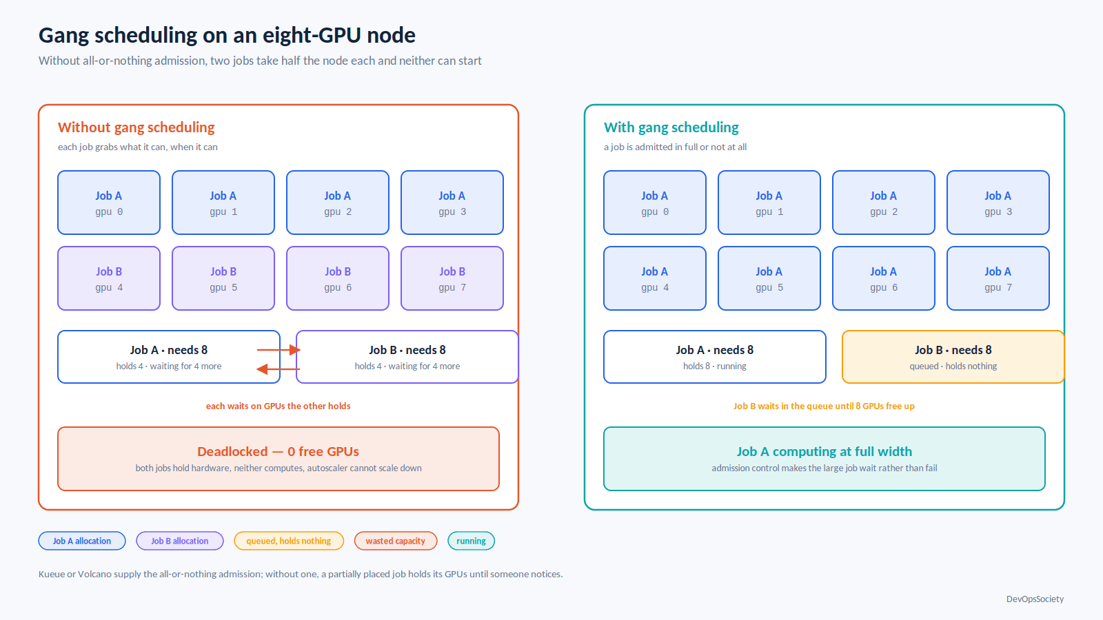
That means admission control, quotas per team, priority classes, preemption of lower-priority work, and gang scheduling so that an eight-GPU job either gets all eight or none. Kueue is the Kubernetes-native option and integrates with Job, JobSet and Ray workloads; Volcano covers similar ground with a batch-scheduler heritage. Without one of them, two eight-GPU jobs will each grab four GPUs, wait indefinitely for four more that the other job is holding, and keep the hardware idle until someone notices.
The model lifecycle: three workloads, three infrastructure profiles
"ML workload" is not a useful category for capacity planning. Training, fine-tuning and inference have almost nothing in common operationally.
Workload | Shape | Hard constraint | What dominates cost | Scheduling model |
|---|---|---|---|---|
Pretraining | Days to months, many nodes, synchronous | Interconnect bandwidth; any node failure stalls the job | Sustained GPU-hours at near-100% occupancy | Gang-scheduled, reserved capacity, checkpoint/restart |
Fine-tuning (LoRA/adapter) | Hours, 1–8 GPUs, one node | GPU memory for optimiser state and activations | Bursty GPU-hours; often spot-eligible | Queued batch, preemptible with checkpoints |
Batch inference / embedding | Minutes to hours, embarrassingly parallel | Data pipeline throughput, not GPU | Total tokens or records processed | Queued, scale-to-zero, spot-friendly |
Online inference (LLM) | Continuous, latency-sensitive | GPU memory for weights plus KV cache | Idle capacity held for peak traffic | Always-on replicas, slow autoscaling |
Online inference (small models) | Continuous, high QPS | Throughput per device | Request volume | Conventional HPA, fractional GPU viable |
The cost model differs from anything in web infrastructure in one specific way: you pay for allocated GPU-hours, not for work done. A GPU held at 15% utilisation costs the same as one at 95%. Utilisation is therefore the headline metric of an AI platform in a way that CPU utilisation never was, and the cost model is the same shape across on-demand, committed-use discounts and reserved capacity you trade flexibility for a lower hourly rate, and the break-even depends entirely on sustained occupancy. Run the provider's calculator against your actual duty cycle before committing to a term.
Training and fine-tuning fit the promotion pattern you already run. A fine-tune that produces a versioned artefact, runs an evaluation suite, and gets promoted on passing thresholds is structurally the same as the commit-to-production path your services already follow, with two differences: the artefact is tens of gigabytes rather than tens of megabytes, and the test suite is statistical rather than deterministic. A model that passes at 91% accuracy and previously passed at 93% is a judgement call, not a red build.
Serving: cold starts measured in minutes
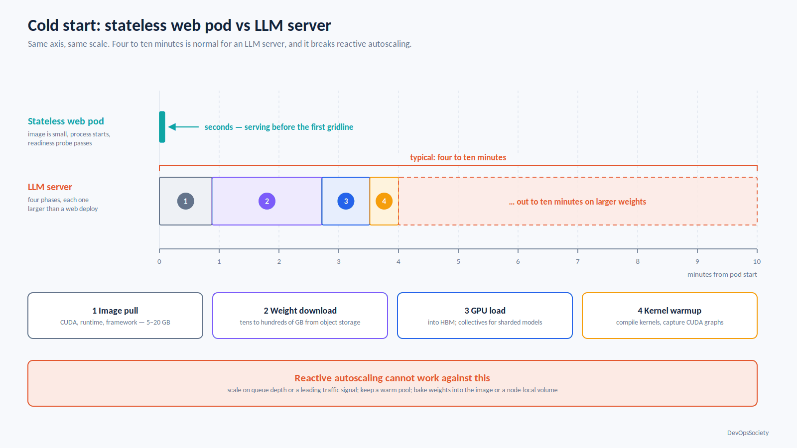
A stateless web container starts in seconds. An LLM server does not, and the reasons stack:
Pull a container image that includes CUDA, a runtime and a framework, typically 5–20 GB.
Download model weights from object storage, tens to hundreds of gigabytes.
Load weights into GPU memory and, for sharded models, establish collectives across devices.
Compile or warm kernels; some runtimes capture CUDA graphs on first requests.
Four to ten minutes is normal. That number breaks reactive autoscaling outright. The mitigations are all unglamorous: bake weights into the image or onto a pre-warmed node-local volume, keep a warm pool sized to your worst plausible spike, use provisioned capacity rather than scale-from-zero for anything user-facing, and scale on queue depth or a leading traffic indicator rather than on observed latency.
For LLM serving specifically, the runtime does most of the work. vLLM, SGLang and TensorRT-LLM implement continuous batching (new requests join the batch mid-flight rather than waiting for a batch boundary) and paged KV cache management, which stops per-request key/value cache from fragmenting memory. The knob you will actually touch is the fraction of GPU memory the server is allowed to claim:
args:
  - --model=/models/llama-3.3-70b-instruct
  - --tensor-parallel-size=4          # shard across 4 GPUs in one NVLink domain
  - --gpu-memory-utilization=0.92     # rest is headroom; too high and you OOM mid-request
  - --max-model-len=16384             # caps KV cache per sequence, so it caps concurrency
Set --gpu-memory-utilization too high and the server dies under concurrency; too low and you are paying for memory you never use. And note that --max-model-len is a capacity control, not just a product setting: longer context means more KV cache per request, which means fewer concurrent requests on the same card.
Observability: your current stack collects none of it
Node exporter tells you nothing about a GPU. You need the DCGM exporter (or your cloud's equivalent) to get the signals that matter: SM occupancy, memory used versus reserved, memory-bandwidth utilisation, power draw, temperature and throttle reasons, ECC error counts, and XID errors.
Learn to read XID errors early. They are NVIDIA's hardware/driver fault codes, and in a fleet of any size you will see GPUs fall over with them. The operational answer is to treat a GPU as a component that fails: node-problem-detector rules that cordon and drain on repeated XIDs, and an automated return-to-vendor path.
For serving, the latency metric you care about splits in two. Time-to-first-token reflects prompt processing and queueing; inter-token latency reflects the memory-bandwidth-bound generation loop. A single p95 across the whole response hides both. Track them separately, along with queue depth and running-batch size, because those are what tell you whether to add replicas.
For training, the metric that matters most is the one nobody instruments: the percentage of wall-clock job time in which the GPUs were actually computing. Data-loading stalls, checkpoint writes and straggler nodes all show up there and nowhere else.
What to do before the first GPU node lands
If you are standing this up now, in order:
Decide the tenancy model first. Whole-GPU per workload is the simplest thing that works. Only reach for MIG when you have measured utilisation low enough to justify the operational cost, and never use time-slicing for anything with an SLO.
Install a queue before you install a second team. Quotas and gang scheduling are much harder to retrofit once people have learned to grab capacity directly.
Instrument utilisation on day one. You cannot argue about reservations, quotas or chargeback without per-team GPU-hours and occupancy.
Separate training and serving pools. They have opposite requirements one tolerates preemption and wants spot capacity, the other cannot tolerate either.
Write down your cold-start budget. It determines whether scale-to-zero is available to you at all, and that single answer drives most of your serving architecture.
The honest caveat: this layer is moving faster than the rest of your platform. DRA only reached GA in Kubernetes 1.34, serving runtimes ship meaningful changes monthly, and the GPU you standardise on this year will be a generation behind within eighteen months. Build the abstractions (queue, quota, artefact promotion, utilisation accounting) to outlive the hardware, and expect to replace the runtime layer more often than you are used to.